Engineering case study
Great Britain's electricity demand moves 13 GW in an ordinary day. GridCast forecasts it half-hour by half-hour.
A full forecasting system built end to end — NESO's 2024 half-hourly record, an engineered feature set, a trained and versioned model artifact, a typed FastAPI service, and an analytics dashboard that reads from all of it.
Held-out week, 18-25 Nov 2024
Worst week of the test split · 1.49% MAPE
Scroll the plot sideways for the full week
Observed national demand against the saved model's prediction for the same half-hour, on data it never trained on. At grid scale the two lines are hard to separate, so the lower panel magnifies the difference. This is the weakest week in the held-out period; the split as a whole comes in at 1.36% MAPE.
- 17,232
- Half-hourly rows · NESO 2024
- 11
- Engineered model features
- 3,447
- Held-out rows · 21 Oct – 31 Dec
- 1.36%
- MAPE, one step ahead
Electricity cannot be stored at grid scale, so supply has to be scheduled against a demand that has not happened yet.
Across 2024, national demand ran from 15.07 GW on an August night to 45.2 GW on a January evening — a threefold spread. A median day swings 12.83 GW between its trough and its peak.
Those swings are fast. The steepest half-hour in the record moves 3,674 MW — eight per cent of the whole year's peak, arriving in thirty minutes. Generation has to be committed before the ramp does, which makes a good short-horizon forecast the input everything else depends on.
15 January 2024 — the year's largest single-day swing
Observed demand · 48 half-hourly settlement periods
21.8 GW between trough and peak on a single winter day. Every point on this curve is a measured value from the NESO record — no model is involved.
Two baselines, one chronological split, and the numbers the artifact actually stores.
The split is by time, not at random: the model trains on 13,785 rows up to 21 October 2024 and is scored on the 3,447 rows that follow. Nothing from the test period is available at training time.
| Model | MAE (MW) | RMSE (MW) | MAPE | R² | State |
|---|---|---|---|---|---|
| Linear Regression | 385.7 | 492.0 | 1.36% | 0.9936 | Saved artifact |
| Random Forest Regressor | 374.4 | 492.2 | 1.29% | 0.9936 | Evaluated |
Both baselines are scored on the same held-out split, and training keeps the one with the lower RMSE: Linear Regression, by 0.15 MW (492.03 vs 492.18 MW). That is the artifact saved and served. Random Forest is slightly better on MAE (374.4 vs 385.7 MW) and MAPE (1.29% vs 1.36%). A gap this small doesn't pick a winner. It's why the model interface is swappable.
The error is centred, not biased
predicted − observed · all 3,447 held-out half-hours
46.6% of half-hours land within 1% of the observed value and 77.4% within 2%, with no systematic tendency to over- or under-forecast.
It is weakest overnight, strongest at peak
mean absolute % error by hour of day
Error peaks at 01:00 (2.86%) and on the 06:00 morning ramp, and falls to 0.65% at the 19:00 evening peak — the half-hours the grid is most sensitive to.
Read this carefully
Every figure above is one step ahead. The feature set includes the previous half-hour's observed demand, so 1.36% MAPE describes the next-half-hour prediction. The dashboard's 48-hour horizon is produced recursively — each prediction is fed back in as the next row's lag — so error compounds across the horizon, and that horizon has not been separately backtested.
Six stages, each with an artifact you can open.
- 01IngestNESO Historic Demand Data 2024, half-hourly settlement periods.17,232 validated rowsbackend/ml/ingestion
- 02EngineerCalendar parts, plus lag and rolling-demand windows at 1, 48 and 336 periods — a half-hour, a day, a week.11 feature columnsbackend/ml/features
- 03SplitChronological 80/20. Random shuffling would leak the future into training on a time series.13,785 train / 3,447 testbackend/ml/training
- 04Train & compareLinear Regression and Random Forest scored on the same held-out window; metrics written beside the model.model.pkl + metadatabackend/models/model_metadata.json
- 05ServeTyped FastAPI endpoints for forecast, history, metrics, model metadata, SHAP explanation and simulation.8 REST endpointsbackend/app/api
- 06PresentNext.js App Router reads the API and refuses to render fallback values as if they were results.6 dashboard viewssrc/lib/page-data.ts
The decision that mattered most: leakage
The raw file ships three demand columns. Transmission System Demand and England & Wales Demand are near-perfect proxies for the target and are recorded at the same instant — including them would have produced a spectacular score and a useless model. Both are dropped, and the metadata says so in writing.
Feature set, in full
- hour
- day
- month
- day_of_week
- is_weekend
- demand_lag_1
- demand_lag_48
- demand_lag_336
- demand_rolling_3
- demand_rolling_48
- demand_rolling_336
Target: ND (national demand, MW). No weather, no holiday flag, no generation mix — the model is a demand-and-time baseline, and the page says so rather than implying otherwise.
Five views over the same artifacts.
Screenshots of the running application — plus a sixth, Schedules, that tracks forecast and training runs. Every view is reachable now, with no sign-in.
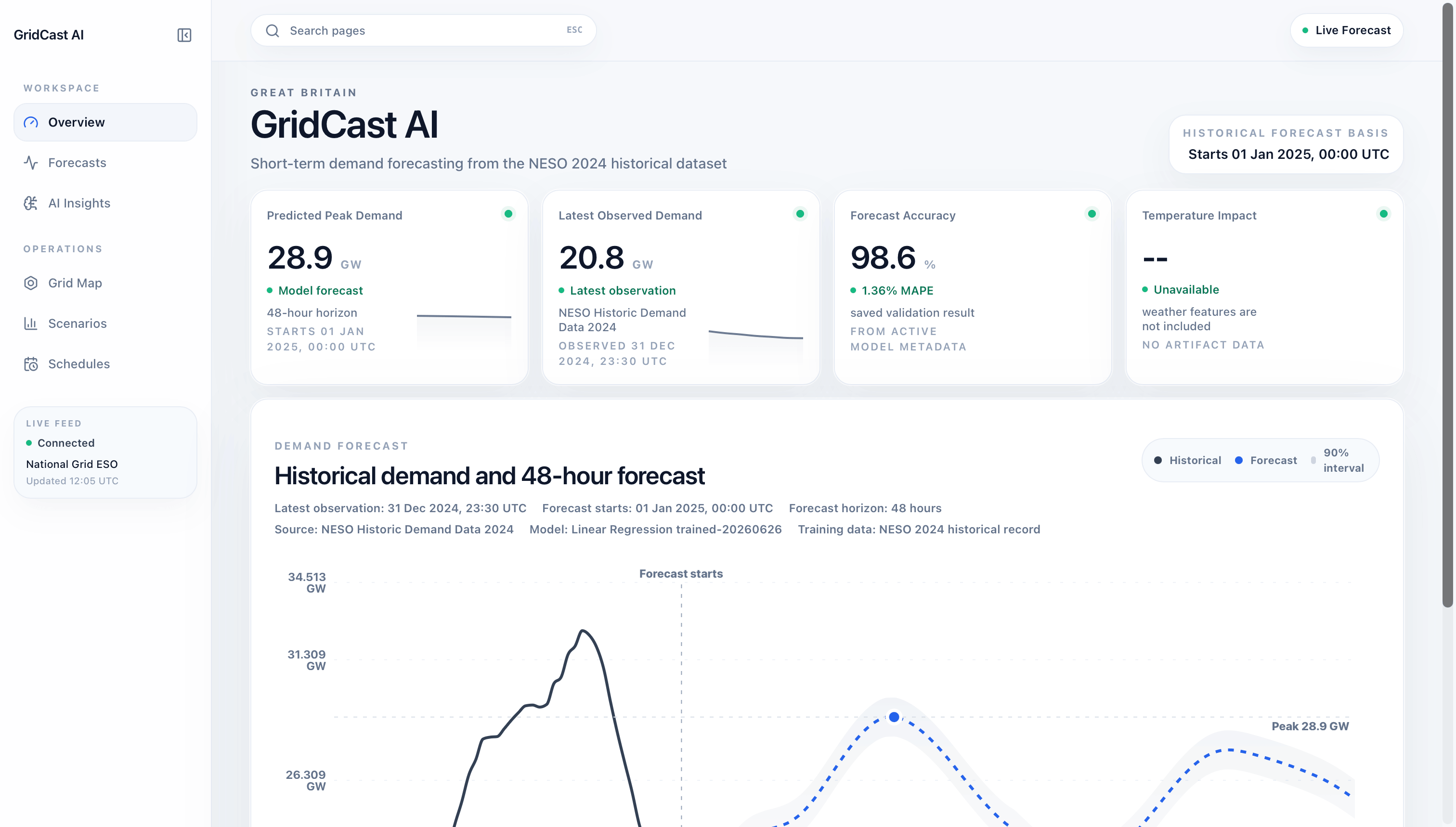
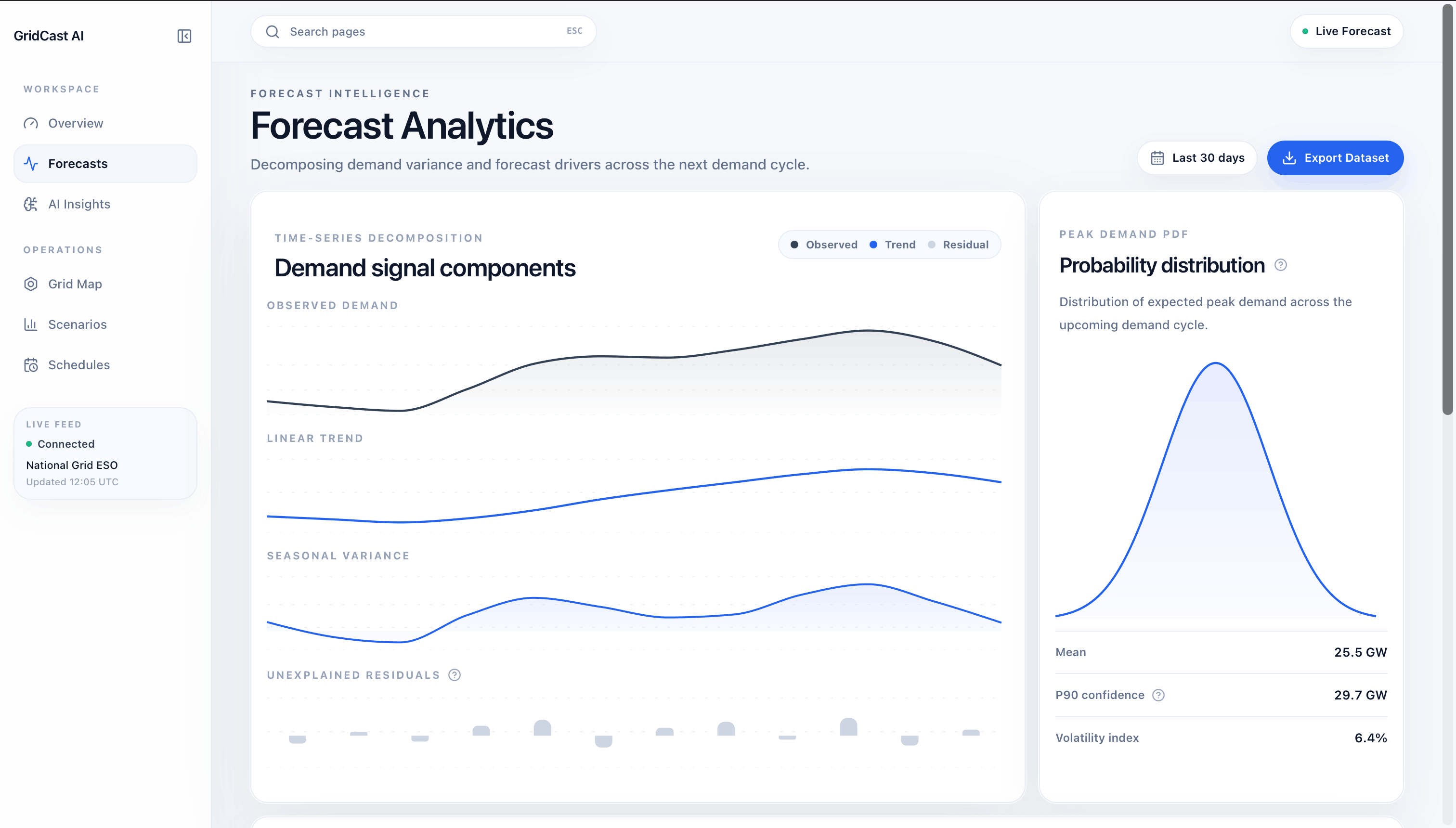
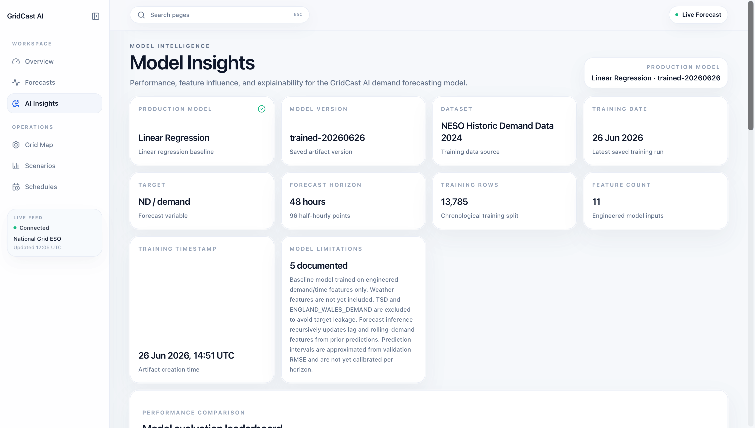
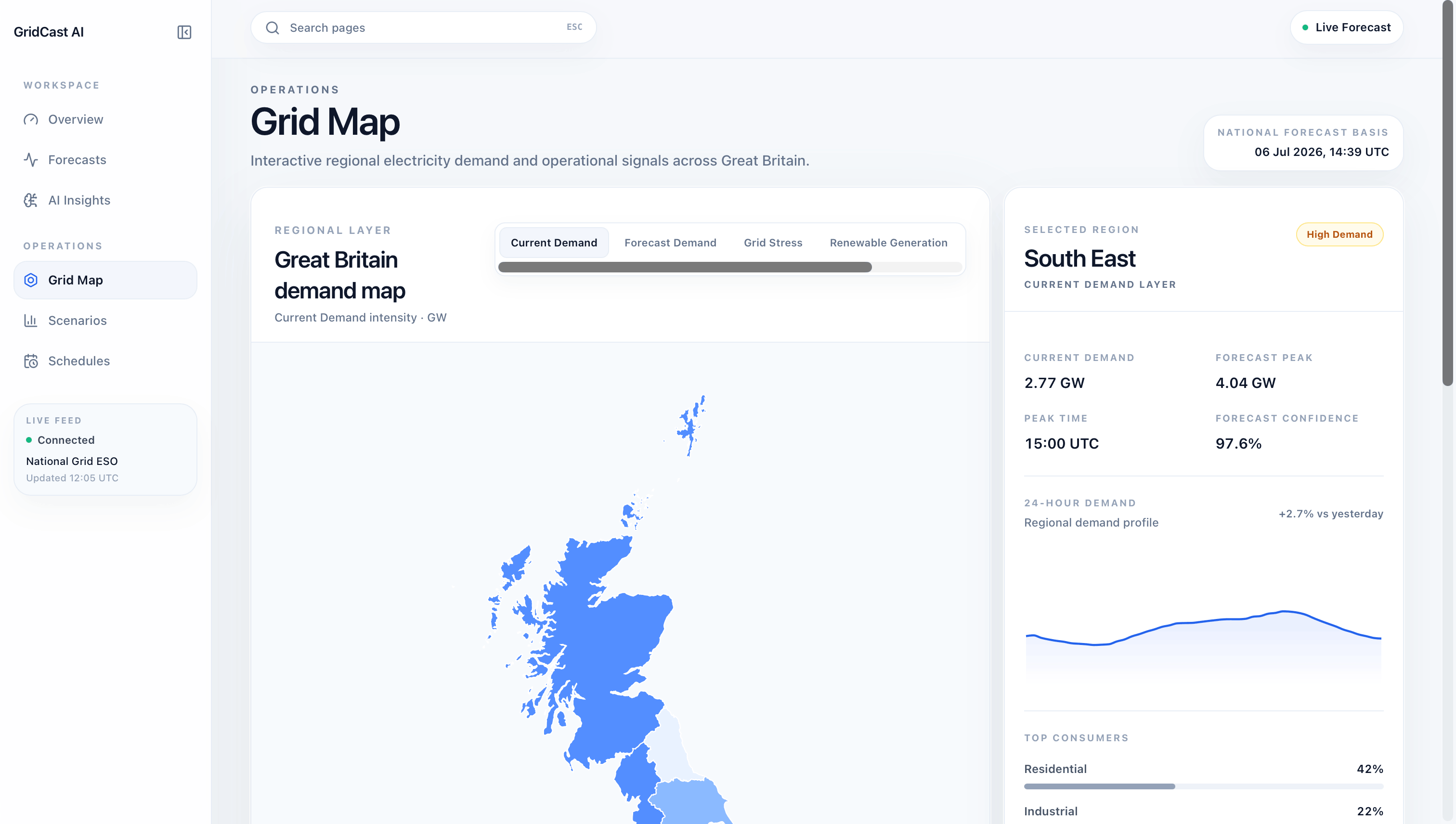
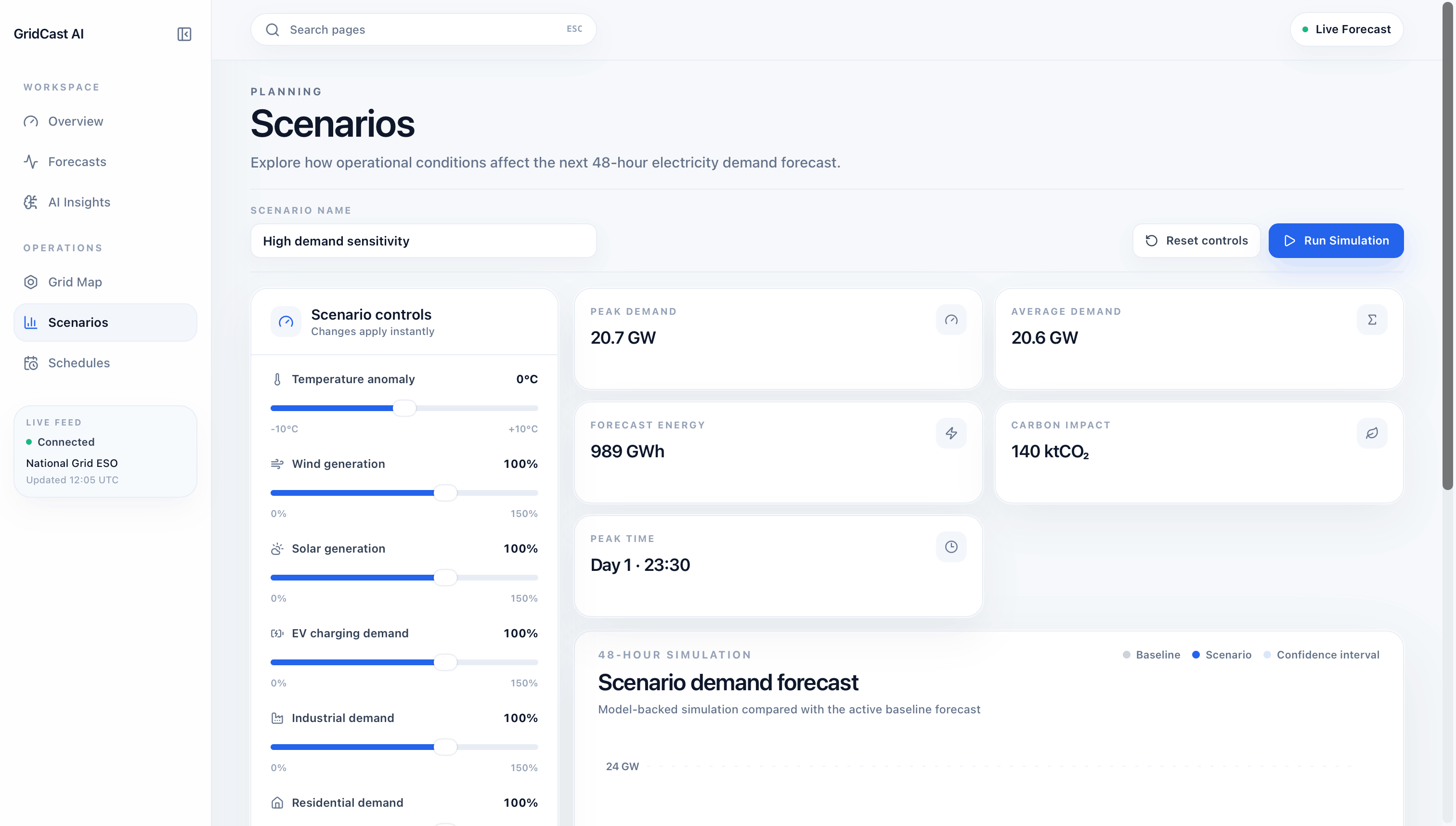
Scroll the frame sideways to read it
Overview. Headline figures come from the saved model artifact and the NESO 2024 dataset; the temperature tile reads “Unavailable” because weather is not a model input.
Open Overview →The limitations are part of the deliverable.
These strings are not marketing copy written for this page. They are stored beside the model and returned by the API, and the dashboard renders the same list. If a value cannot be sourced from a real artifact, the UI shows Unavailable instead of a placeholder.
What would close them
Rolling-origin backtesting
measures the 48-hour horizon, not just one step
Live NESO ingestion
replaces the frozen 2024 file with a running feed
Weather ingestion
the largest missing driver of demand
Probabilistic forecasting
calibrated intervals instead of an RMSE proxy
XGBoost + LSTM comparison
a third and fourth entry on the leaderboard
Planned work, listed in the repository README. None of it is implemented yet.
Model · documented in model_metadata.json and the API
- Baseline model trained on engineered demand/time features only.
- Weather features are not yet included.
- TSD and ENGLAND_WALES_DEMAND are excluded to avoid target leakage.
- Forecast inference recursively updates lag and rolling-demand features from prior predictions.
- Prediction intervals are approximated from validation RMSE and are not yet calibrated per horizon.
Scenario simulator · documented in simulation_service.py
- Temperature, generation mix, sector demand, and bank holidays are not dedicated features in the current model.
- Those inputs currently use isolated provisional adjustments to lag and rolling-demand features.
- Lag and rolling values are held from the latest observation rather than updated recursively.
Scope
- Forecasts run from the saved 2024 dataset and model artifact. There is no live NESO feed.
- The 48-hour recursive horizon has no rolling-origin backtest yet, so only one-step-ahead error is measured.
- Regional map layers allocate the national forecast by fixed shares; the model is not regional.